Learn how to use Excel’s most commonly used Function VLOOKUP, explained in the easiest way and also visually so that you understand it well!
Excel VLOOKUP Function searches for the value you specify and returns a matching value from another column. More technically, the VLOOKUP function looks up a value in the first column of the specified range and returns a value in the same row from another column.
In its common usage, Excel VLOOKUP searches through your data set based on the unique identifier and brings you information associated with that unique identifier.
Official VLOOKUP Syntax as explained by Microsoft:
Summary
VLOOKUP Function is an Excel function to lookup and retrieves data from a specific column in the table. VLOOKUP supports approximate and exact matching and wildcards (* ?) for partial matches. The “V” stands for “vertical”. Lookup values must appear in the first column of the table, with lookup columns to the right.
Purpose
Lookup a value in a table by matching on the first column
Return value
The matched value from a table.
Let’s understand the Excel VLOOKUP function with an easy example:
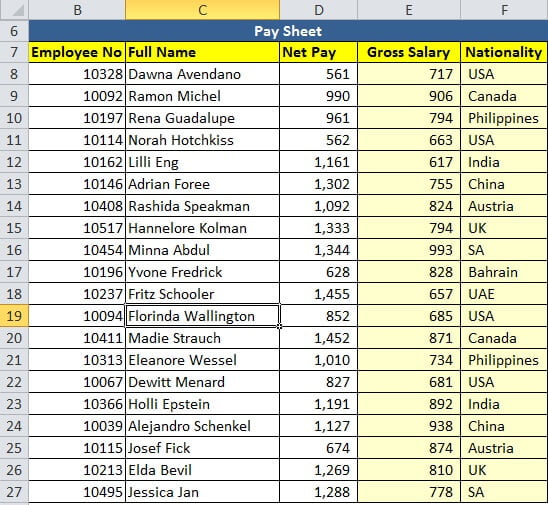
Suppose We have employees’ Paysheet report, as you can see below.
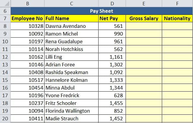
For the reference, we will call above paysheet table as Report table. We want to retrieve Gross Salary (Column E) and Nationality (Column F) of by employee number (Column B) from another location which would be our Lookup Array or Lookup Table which you can find below:
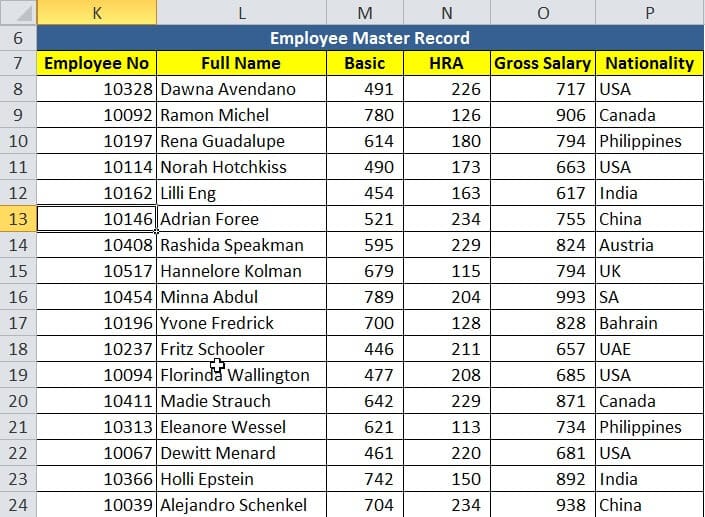
For the references, we would call above table range as a Lookup table. From this lookup range or table, we are looking for Gross Salary and Nationality employee wise.
Lets see how VLOOKUP syntax is applied to our example. Below is step by step animation how VLOOKUP ‘s arguments flows:
From the above animation, we can see that what are the arguments with our examples. Please note that the first three arguments are compulsory and the fourth argument is optional which is the type of match we are looking for.
By default, VLOOKUP function applies 1 or TRUE or Approximate match (I will explain you Approximate matches and wildcards in another post). But we are looking for an Exact Match in this scenario, so we will be selecting either FALSE or 0.
Below is another image showing VLOOKUP Formula explained in both Report table and Lookup table to reinforce the formula syntax concept:
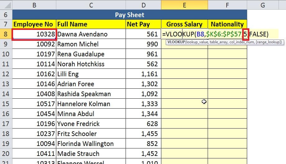
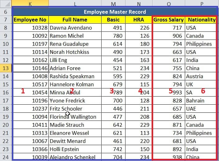
Column Index number will be 6 instead of 5 when we would write the formula in Nationality column in Report table (paysheet, left the table).
Please note that we can also select table array till column O instead of P since we are looking for Gross Salary in Report table in column E, but since we want table array to be consistent we should select full table array till column P.
The completed table after the formula is written will look like as follows (Report Table/Paysheet)
Video Tutorial from my YouTube Channel, Do not forget to subscribe my YouTube channel for excellent basic to advance Excel tutorials FREE!
Following are key points to remember while using VLOOKUP Function (Caution)
- VLOOKUP always looks up values from Left to Right, it is not capable of looking values from right to left, so in above example, if employee number was in the second or third column in our Lookup table/lookup array/Master records table, VLOOKUP function would not have worked (Index and Match Function together would be the best option, I will cover them in different post). In other words, the Lookup value column MUST be the very first column in our Lookup array range or table.
- Excel VLOOKUP is case-insensitive, meaning that uppercase and lowercase characters are treated as equivalent.
- Lookup values should always be unique parameters in Lookup Array (range/table), otherwise, Vlookup will only return the first matching value.
- In above example, if we were to look up for Nationalities of employees as Lookup value instead of Employee number, Vlookup would return first matching value corresponding to the Nationality value, eg if there were two employees with USA nationality, VLOOKUP would return first one only and rest USA nationality employees would be ignored.
Besides the above limitations, if you follow VLOOKUP rules strictly, it is quite handy and powerful Excel Function, and helpful in creating Dashboards and reports on the go!
If you have found this post and tutorial useful, please do not forget to share it with your friends and colleagues. Also, share it on social media!
As promised I will do one more post covering VLOOKUP advanced functionalities, so stay tuned and subscribe to my newsletter so that you won’t miss the tutorial.
One Response
wonderful Prashant.